Everything Lies: Gyro Drift

Gyroscopes lie

Any person getting into robotics has heard the phrase:

Gyroscopes drift. You can’t trust them.

But what does that actually mean?

A gyroscope measures angular velocity. If you integrate that measurement over time, you get orientation. So in theory, if a robot starts perfectly level and doesn’t move, the gyro should continue reporting zero rotation forever.

Except it doesn’t. If you leave an IMU sitting on a table, and after a while it will confidently tell you that it has rotated several degrees. The robot hasn’t moved. The room hasn’t moved. The sensor has simply accumulated a small error until it has invented a completely different reality.

But IMUs are everywhere. Your phone, drones, autonomous vehicles, industrial robots, spacecraft, game controllers… Almost every modern system that needs to understand motion uses them. If gyroscopes are so unreliable, how can industry depend on them?

The answer is that we don’t expect sensors to tell the truth. We expect them to lie predictably.

How do they lie?

I am not going to bore you with the details of the inner mechanical workings of a gyroscope sensor. That can be (and is) the topic of many pages (such as this one) which I implore you to read.

However, for the purposes of this blog post what you need to understand is that gyros measure angular velocity ($\omega$) and have two sources of ‘error’: measurement noise and bias (or drift).

Measurement noise

This is the easier one to understand, so let’s start with it.

Measurement noise is the random variation in a sensor’s output even when the true value has not changed.

Imagine placing a gyro perfectly still on a table. The true angular velocity is 0.

However, the sensor might report:

0.02 deg/s
-0.01 deg/s
0.03 deg/s
0.00 deg/s
-0.02 deg/s

The sensor is not consistently wrong. It is just noisy. This can be from quantization, EMI, thermal noise, really anything.

This kind of error is usually well behaved. If you take enough measurements and average them, the noise tends to cancel out.

This is why filtering works well for measurement noise.

We can model this as zero mean additive gaussian noise, $n_k$.

Bias

This error is far more insidious.

Unlike noise, bias is a consistent error in the sensor’s measurement. Instead of randomly fluctuating around the true value, the sensor has a small offset.

Imagine the same gyro, sitting perfectly still, reporting:

0.05 deg/s
0.05 deg/s
0.06 deg/s
0.05 deg/s
0.04 deg/s

The sensor is just plain wrong.

This is much harder to deal with because taking more measurements does not help. Averaging a thousand noisy measurements might get you closer to the true value, but averaging a thousand biased measurements simply gives you a more accurate estimate of the wrong answer.

What’s worse is that this bias is not constant either. It floats up and down.

Imagine flipping a coin. Heads, you take one step forward. Tails, you take one step back. After 100 flips, you could be at -20, +7, +35, or really anywhere depending on how the coin landed.

The bias behaves similarly. It doesn’t steadily increase or steadily decrease; instead, it slowly wanders over time.

This process can be modelled as a random walk (for short periods. Though it’s not entirely accurate, it’s good enough for our purposes. Look into Ornstein–Uhlenbeck processes for a more accurate model of gyro bias).

A random walk is a stochastic process where the current value is equal to the previous value plus some random perturbation:

\[x_k = x_{k-1} + w_k\]

Where $w_k$ is generally modelled as zero mean gaussian noise. In the example given above, it would be how far forwards or backwards we walk at each step.

Using the same model for our bias term $b_k$:

\[b_k = b_{k-1} + w_k\]

Basically, our bias right now is the bias we had earlier, plus a small offset.

The full measurement model

Putting the two sources of error together, we get a model that looks like:

\[\omega_m = \omega + n + b\]

Where:

• $\omega_m$: Measured angular velocity
• $\omega$: Real angular velocity
• $n$: Measurement noise
• $b$: Gyro bias

The devil: Integration

Now, you may be thinking that doesn’t sound so bad. I mean, all measurements have a bit of noise, right? What’s the big deal?

Dear reader, I’ll tell you what the big deal is. You’re right. It’s not a huge issue if you’re using angular velocity. But most people don’t want angular velocity. They want orientation.

A gyroscope doesn’t measure orientation directly. It measures angular velocity, so to recover orientation we have to integrate:

\[\begin{aligned} \omega &= \frac{d\theta}{dt} \\ \implies \theta &= \int_0^t\omega \ dt + \theta_0 \tag{1} \end{aligned}\]

Where:

• $\theta$: Current orientation
• $\theta_0$: Reference orientation (at $t=0$)
• $\omega$: Angular velocity

But this doesn’t take noise into account. Subbing $\omega \rightarrow \omega_m$ into $(1)$:

\[\begin{aligned} \theta_m &= \int_0^t\omega_m \ dt + \theta_0 \\ & = \int_0^t \omega + n + b \ dt + \theta_0 \\ &= \underbrace{\int_0^t \omega \ dt + \theta_0}_{\theta} + \int_0^t n \ dt + \int_0^t b \ dt \\ \end{aligned} \\ \boxed{\theta_m = \theta + \int_0^t n \ dt + \int_0^t b \ dt}\]

The orientation estimate now contains every error the gyro has ever made.

The first error term,

\[\int_0^tn\ dt,\]

is the accumulated measurement noise. Even though the instantaneous noise is zero-mean, integrating it causes the orientation estimate to perform an angle random walk.

The second term,

\[\int_0^tb\ dt,\]

is the accumulated bias. This is even more troublesome. A constant bias produces a linearly growing orientation error, while a slowly varying bias causes the estimate to drift unpredictably over time.

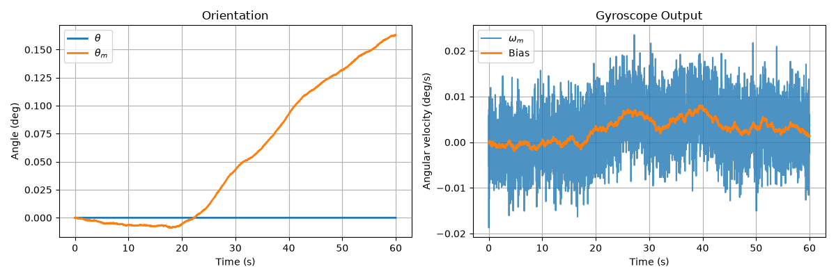
The effect is much easier to appreciate in simulation. Below, the true orientation remains fixed while the estimated orientation slowly wanders away, despite the gyro errors appearing almost insignificant.

The patchwork solution: Calibration

At this point, the obvious question is:

“If the gyro is wrong, why don’t we just measure how wrong it is and subtract the error?”

And that is exactly what calibration does.

A simple gyro calibration procedure is:

Keep the sensor completely still. Collect a large number of measurements. Average the measurements. Use this average as the bias correction.

Since the true angular velocity is zero while the sensor is stationary:

\[\omega_m = 0 + b + n\]

Taking the average over many measurements gives:

\[\bar{\omega_m} \approx b\]

because the zero-mean noise term tends towards zero: \(\bar{n} \rightarrow 0\) So we can estimate the bias and subtract it during operation:

\(\omega_{corrected} = \omega_m - \hat{b}\) Problem solved, right?

Well… let’s try.

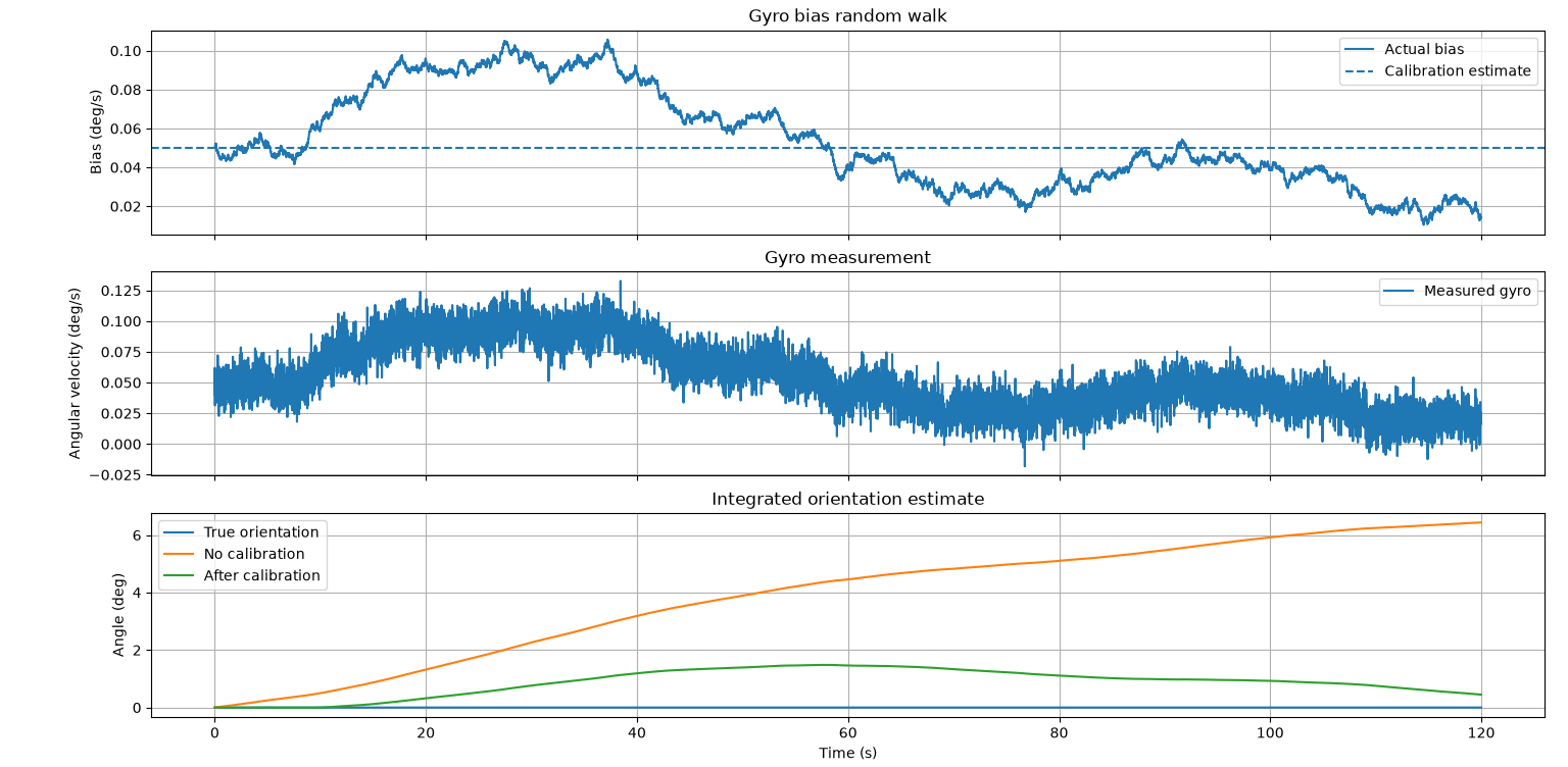
This is significantly better. However, it is still not a complete solution.

The problem is that we assumed something that isn’t true: that the bias is constant. Calibration removes the bias that existed during the calibration process, but it cannot predict how the bias will change later.

Introducing the accelerometer

This solution is a little more involved. Instead of relying only on the gyro, we use more information from the IMU. Specifically, the accelerometer.

The key observation is that gravity gives us a reference vector.

When the sensor is stationary, the only acceleration acting on it is gravity. This means the accelerometer will measure:

\[a \approx g\]

where $g$ points towards the centre of the Earth.

From this, we can estimate the sensor’s orientation relative to gravity.

For example, if the accelerometer measures:

\[a = \begin{bmatrix} 0 \\ 0 \\ 9.81 \end{bmatrix} ​\]

the sensor is likely level. If gravity appears along the X-axis instead, the sensor has rotated.

Unlike the gyro, this measurement does not suffer from integration drift when used to estimate orientation. A gyro can accumulate error forever, but the accelerometer always provides an external reference for tilt.

However, the accelerometer has its own problem.

It cannot distinguish between gravity and acceleration caused by motion.

If the robot accelerates forward, the accelerometer sees:

\[a_{\text{measured}}=a_{\text{motion}} + g\]

It has no way of knowing which part came from gravity and which part came from the robot moving.

So we have two imperfect sensors:

The gyro is excellent at measuring short-term changes, but drifts over time. The accelerometer provides a long-term reference, but becomes unreliable during motion.

The complementary filter fuses these two sensors, using the best bits from both.

The complementary filter

What we’re going for is this:

I trust the gyro for what happened recently, but I periodically pull my estimate back towards what gravity says

The way that this is achieved is mind bogglingly simple.

We take the two estimates of orientation:

• The gyro estimate, obtained by integrating angular velocity.
• The accelerometer estimate, obtained from the direction of gravity.

Then we take a weighted average:

\[\theta = \alpha\theta_{\text{gyro}} + (1-\alpha)\theta_{\text{acc}}\]

where:

\[0 < \alpha < 1\]

The value of $\alpha$ determines who we trust more.

If:

\[\alpha = 1\]

we completely trust the gyro. We get a fast response, but drift forever.

If:

\[\alpha = 0\]

we completely trust the accelerometer. We never drift, but every acceleration looks like a rotation.

A practical value might be:

\[\alpha = 0.98\]

meaning:

• 98% of the estimate comes from the gyro.
• 2% comes from the accelerometer.

At first this seems like a poor compromise. Why only give the accelerometer 2% influence? But since we apply this correction continuously, the accelerometer gets another small opportunity to correct the gyro drift at every timestep.

However, recall that the measurement from the gyro is angular velocity, not orientation, so instead of integrating based on the noisy value, why don’t we use the cleaner, filtered version? Then $\theta_{\text{gyro}}$ just needs to be updated every timestep.

Hence, we use the recursive form of the complementary filter:

\[\theta_k = \alpha(\theta_{k-1} + \omega_k \Delta t) + (1-\alpha)\theta_{\text{acc, }k}\]

Let’s try! For this demo, I have made the sensor move. Otherwise this is actually just perfect.

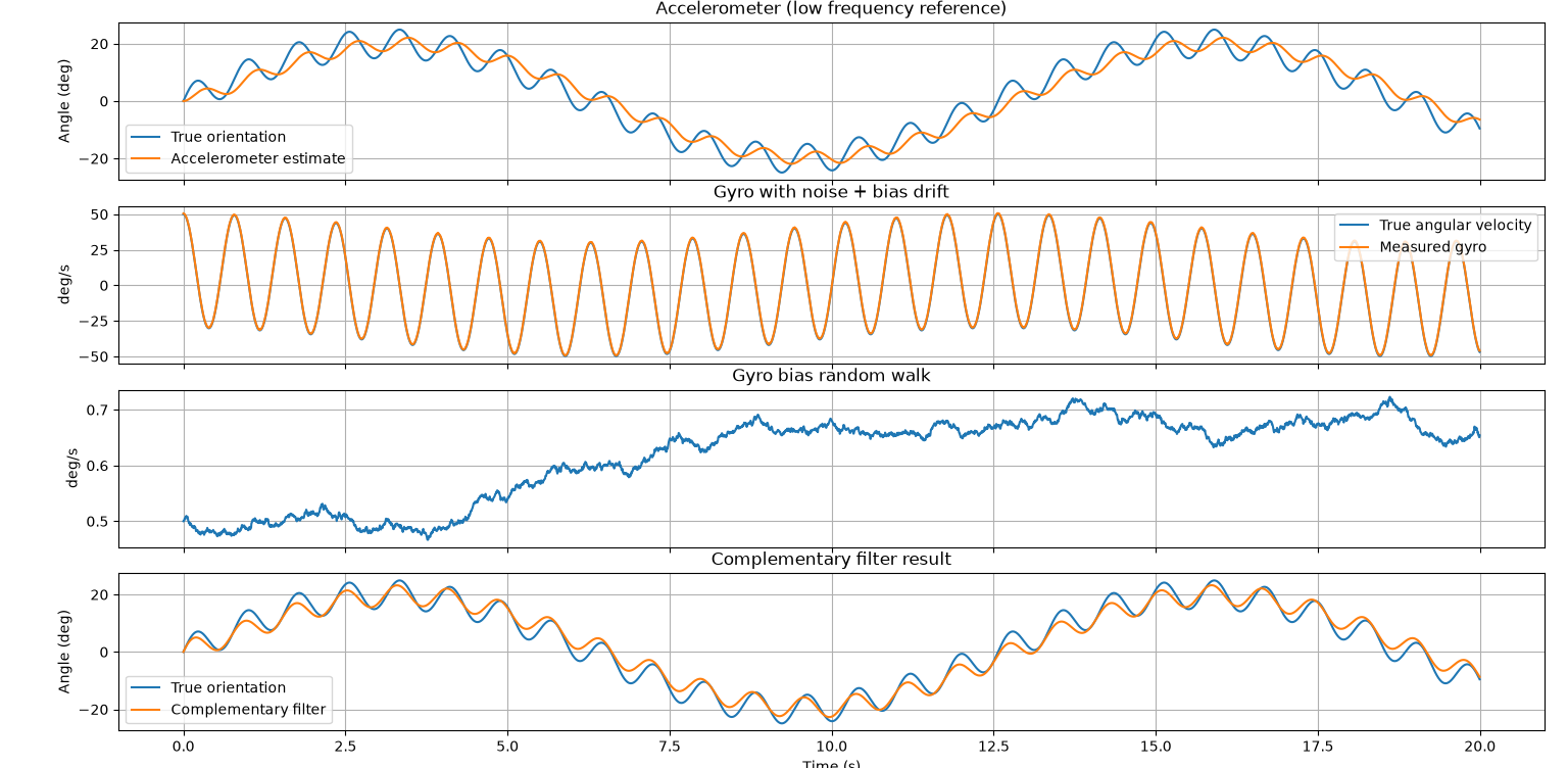
Okay, this is substantially better. It’s actually able to track, and stays on target! However, we can see that it’s not perfect. When the orientation changes quickly, it can’t keep up. Let’s try varying $\alpha$.

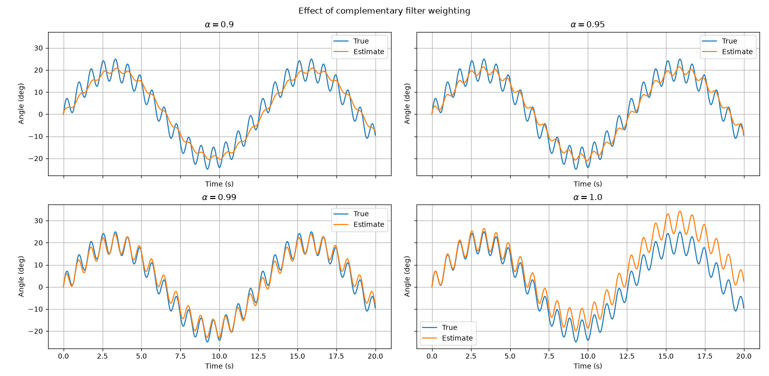
It’s interesting. For lower $\alpha$, it’s almost like the high frequency rotations are being treated like noise. Also, notice that for $\alpha = 1$, the estimated orientation just drifted off the actual one.

Furthermore, notice that for lower values of $\alpha$, the peaks of the waves are offset. The estimate appears to lag behind the true orientation.

This is a consequence of the low-pass behaviour of the accelerometer correction. By trusting the accelerometer more, we are effectively smoothing the estimate more aggressively. This removes high-frequency noise, but also introduces phase delay.

For this test, $\alpha = 0.99$ is probably best. However, this is the issue with the complementary filter. It needs to be calibrated per application.

That’s not the biggest deal honestly, and most hobby or early prototype-level projects probably don’t need anything more complicated than a complementary filter.

But there is a fundamental limitation: the filter has no idea whether the gyro or accelerometer is currently trustworthy. The value of $\alpha$ is fixed.

What happens if the robot is accelerating and the accelerometer becomes unreliable? What happens if the gyro temperature changes and its bias increases?

We need a filter that doesn’t just combine measurements, but estimates how much we should trust each measurement. This is (drum roll please) the Kalman filter.

Enter: Kalman

I will not go super in-depth into the Kalman filter. You can refer to this previous blog post for more details and derivations.

If you don’t want to do that (please do it), the general gist of the Kalman filter is this:

Instead of manually deciding how much to trust each sensor, the Kalman filter keeps track of how uncertain each measurement is and adjusts the weighting automatically.

Remember our complementary filter:

\[\theta_k = \alpha(\theta_{k-1} + \omega_k\Delta t) + (1-\alpha)\theta_{\text{acc},k}\]

The value of $\alpha$ was fixed. We decided beforehand that the gyro gets 99% trust and the accelerometer gets 1% trust.

But what if the robot is accelerating?

The accelerometer is no longer just measuring gravity:

\[a_{\text{measured}} = a_{\text{motion}} + g\]

Our accelerometer estimate is now unreliable. A good estimator should reduce its trust in the accelerometer.

Likewise, if the gyro heats up and its bias starts changing faster, the estimator should notice that its prediction is becoming less reliable.

This is the key idea behind the Kalman filter:

Don’t decide how much to trust a measurement beforehand. Estimate how much to trust it while running.

The Kalman filter does this by maintaining a state estimate and an uncertainty estimate.

For our IMU example, the state might be:

\[x = \begin{bmatrix} \theta \\ b_g \end{bmatrix}\]

where:

• $\theta$ is the current orientation.
• $b_g$ is the gyro bias.

The filter continuously does two things:

1. Predict: Use the gyro to predict where we should be.
2. Correct: Use the accelerometer to correct the prediction.

The correction is weighted based on uncertainty. If the accelerometer is unreliable, the Kalman filter mostly ignores it. If the gyro prediction has become uncertain, it gives the accelerometer more influence.

This is one of the biggest advantages over simple calibration. The Kalman filter does not just estimate orientation. It estimates the hidden causes of error. In this case, it can estimate the gyro bias itself and continuously compensate for it.

Again, this is a very high level overview. Please check the aforementioned previous blog post for more detail as to how the Kalman filter actually works.

Anyway, back to the simulator to see how well this works!

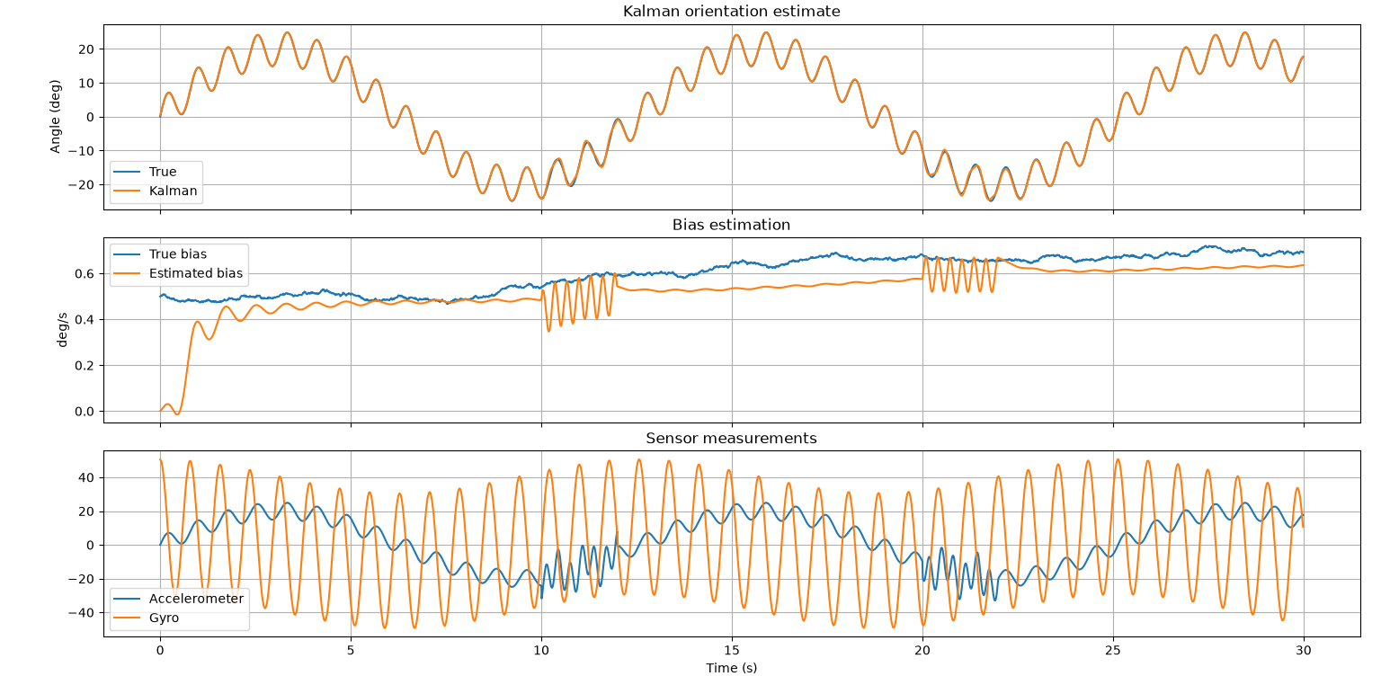
Now, this isn’t perfect either. You can see when there is some acceleration, the estimate becomes worse. However, it is leagues ahead of the complementary filter, and even further than simple calibration.

In conclusion…

I want to show you a comparison of all of these approaches, given the exact same motion.

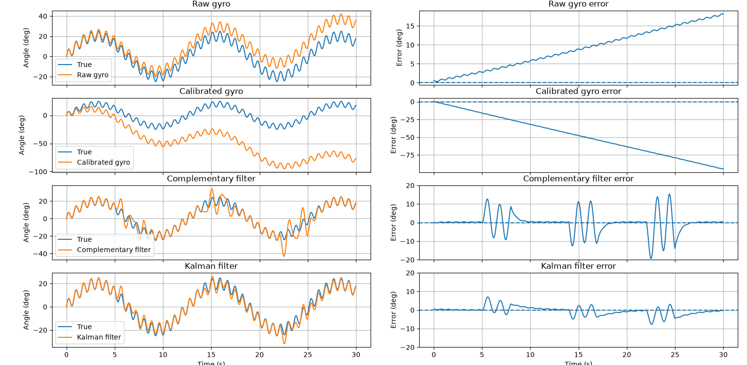
The raw gyro is, unsurprisingly, terrible. The bias error accumulates over time, and because we are integrating angular velocity, even a tiny error eventually becomes a huge orientation error.

The calibrated gyro is an interesting case. You might expect it to perform much better. After all, we measured the bias and removed it. However, remember that the bias is not constant. The calibration only removes the bias that existed at the start of the experiment. As the gyro bias continues to wander, the error slowly comes back.

The complementary filter and Kalman filter both perform significantly better. Both are able to use the accelerometer as an external reference, preventing the estimate from drifting away forever.

However, there is an interesting difference. The errors occur at roughly the same points in time. This makes sense. Both filters are being affected by the same underlying problem: the accelerometer is being corrupted by acceleration, so the gravity estimate becomes temporarily unreliable.

But the difference is the magnitude of the error. The Kalman filter consistently has smaller errors, roughly half that of the complementary filter in this example.

Since the complementary filter has a fixed trust value. It always applies the same correction:

“Trust the accelerometer by 2%.”

It has no idea whether the accelerometer is currently measuring gravity or a large acceleration.

The Kalman filter on the other hand, keeps track of uncertainty. It estimates the gyro bias and adjusts how much it trusts each measurement based on the expected error. It is not that the Kalman filter has found a sensor that tells the truth. It hasn’t. It’s just better at using the information it has.

What comes next?

The Kalman filter feels like the end of the story. We have a model of the system, we have multiple sensors, and we can estimate the hidden state.

But there is a problem. We have only solved one piece of the puzzle: orientation.

A robot does not just need to know which way it is pointing. It needs to know where it is.

A gyro can drift. Wheel encoders can slip. GPS can disappear or become inaccurate (or not even exist underwater!). Every sensor we use to estimate position has its own way of lying.

The next question is no longer:

“How do I estimate my orientation?”

It becomes:

“How do I know where I am?”

That leads us into dead reckoning, odometry, localization, and eventually the world of SLAM.